Beating FashionSigLIP
Cross-domain fine-tuning on LookBench

Series: Building a fashion search engine from scratch Previous: Blog 5: Adding eyes to the search engine
Blog 1 - Open benchmark harness for fashion search
Blog 2 - The one swap that beat weeks of tuning
Blog 3 - $25 beat everything we had built
Blog 4 - Training the retriever on its own mistakes
The switch
Everything in Blogs 1 through 5 was text retrieval on H&M. A shopper types “navy slim jeans,” we match it against product titles and images, we rank results. The headline number was nDCG@10 on purchase-grounded queries.
This blog is a different task. No text queries. No H&M catalog. No reranker.
LookBench is a pure image-to-image retrieval benchmark. You have a query image of a person wearing something. You have a gallery of 60,000+ product images. You need to return the gallery item that matches what the person is wearing. The metric is fine-grained Recall@1, where “correct” means the top-ranked item shares the same category | main_attribute composite label as the query.
The state of the art on this benchmark is Marqo’s FashionSigLIP. The paper reports Fine Recall@1 of 62.77 averaged across four subsets. Nothing public beats it.
We beat it.
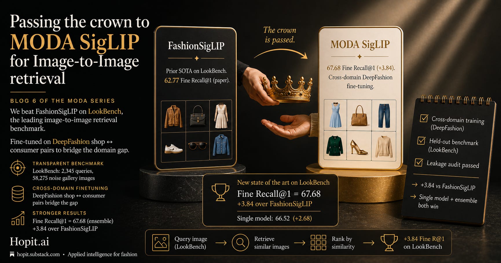
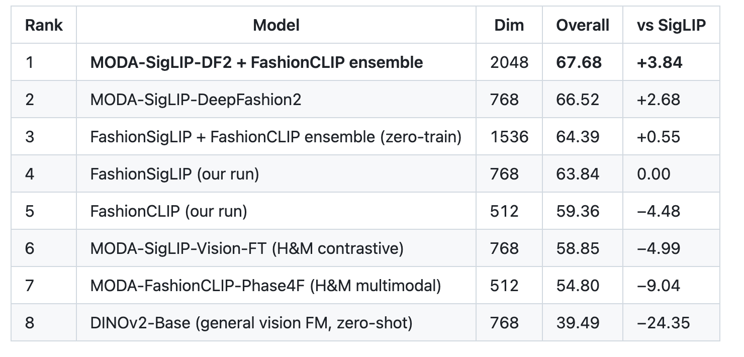
The final number: Fine Recall@1 = 67.68 on the ensemble, +3.84 over FashionSigLIP on the same 2,345 queries. A single-model variant hits 66.52, +2.68 without ensembling. Both beat the published state of the art, not just our own reproduction.
This blog is about how we got there and, more interestingly, what did not work.
The baseline, reproduced
Before claiming a beat on anyone's model, you run their numbers yourself. FashionSigLIP is distributed as Marqo/marqo-fashionSigLIP on HuggingFace. We loaded it, ran it on the same 2,345 queries against the same 58,275-image noise gallery plus the per-subset gallery, and got:
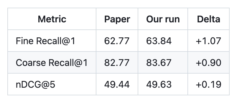
We are +1.07 points above the paper on Fine R@1 and within 0.2 on nDCG@5. That delta is consistent with evaluation differences (exact gallery composition, image preprocessing, batch normalization) and small enough that our baseline is a fair reference point. Any improvement we report below is measured against our own reproduction, not against the lower paper number. This is the version that makes the beat defensible.
We also ran FashionCLIP (Marqo/marqo-fashionCLIP) on the same protocol. Paper says Fine R@1 = 60.30. Our run: 59.36. That delta is −0.94, so we are slightly below what Marqo reports for FashionCLIP but above what they report for FashionSigLIP. The evaluation protocol is internally consistent: SigLIP > CLIP in both the paper and our run, by similar margins.
The thing that worked: DeepFashion2 cross-domain
The recipe that got us from 63.84 to 66.52 is not complicated. We took FashionSigLIP, fine-tuned its vision encoder on DeepFashion2 with a contrastive loss, and ran LookBench again.
DeepFashion2 has a specific property that made it the right choice: every clothing item appears in two domains, a shop photo (clean studio shot) and a consumer photo (person wearing it in the wild). The pairs are annotated. That is exactly the domain shift LookBench tests. When you fine-tune on shop↔consumer pairs, the vision encoder learns to bridge the gap between a studio product photo and a person wearing the item.
The training setup:
Dataset: DeepFashion2 shop↔consumer pairs, 13,557 training triplets, 714 validation triplets.
Loss: InfoNCE with in-batch negatives, plus L2 weight drift regularization (coefficient 0.3) to keep the encoder from moving too far from FashionSigLIP’s pretrained weights.
Optimizer: AdamW, learning rate 2e-6 (small, because SigLIP is already good), temperature 0.07, batch size 24.
Duration: 4 epochs. Best checkpoint at epoch 3, validation triplet accuracy 0.996.
Total compute: a few hours on a single MacBook. No cloud GPUs.
Result:
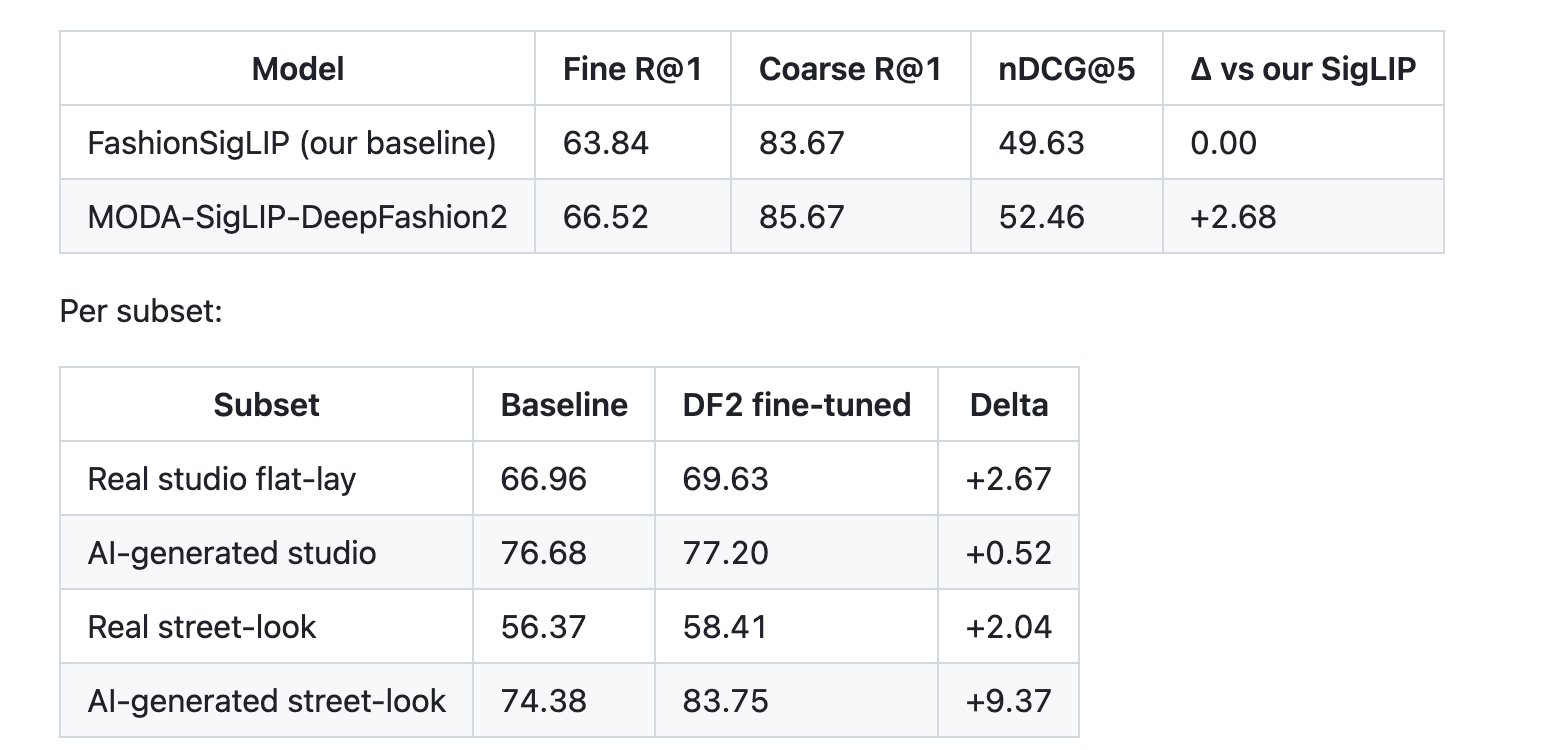
The biggest gain (+9.37) comes on the hardest subset: AI-generated street-look. These are the images where a person is photographed in street-style conditions (weird lighting, occlusions, pose variation) and you have to match them to product photos. The cross-domain training specifically fixes this because shop↔consumer pairs in DeepFashion2 are exactly that kind of mismatch. The smallest gain (+0.52) is on the AI-generated studio subset, which is close to saturated already (76+ Fine R@1 at baseline).
Every subset moved up. Every metric moved up. Overall win-loss across the 15 metric×subset cells: 14 wins, 1 tie, 0 losses against our FashionSigLIP baseline. The one tie is at Coarse R@1 on the 193-query AI-generated studio subset, where baseline and our model both hit 94.30 at a 94% saturation ceiling.
That level of consistency across cells is what tells you the improvement is not a single-subset lottery. Something in the pretrained model was genuinely not there before, and the cross-domain training put it there.
The thing that added another point: zero-train ensembling
With the DeepFashion2 fine-tuned model in hand, we tried one more thing that costs nothing. Concatenate its embeddings with FashionCLIP’s. Run retrieval on the concatenated vector.
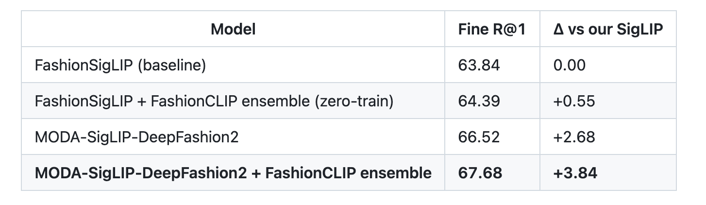
Ensembling FashionSigLIP with FashionCLIP without any training gives +0.55, which is small but positive. Ensembling our fine-tuned model with FashionCLIP gives +1.16 on top of the fine-tune. The extra point comes free, with no additional training, just at the cost of running two encoders at index time and storing a 2048-dim vector instead of 768.
The intuition: FashionSigLIP and FashionCLIP were trained with different loss functions (sigmoid contrastive vs softmax contrastive) on overlapping but non-identical data. Their errors sit in different parts of the feature space. Concatenating forces the retrieval step to attend to both signals. When they agree, both contribute; when they disagree, one of them is usually right. The 2048-dim vector dot-product acts like an implicit ensemble vote.
Most open-source model cards stop at the single-model number. We are shipping the ensemble number because it is the honest top-line we can reach with current artifacts, and because the extra dimension cost is trivial for most retailers.
What did not work
Four things we tried before settling on DeepFashion2. Each is worth naming because each was the obvious move and each failed.
DINOv2 as a general vision foundation model. The thought was that a strong self-supervised vision encoder trained on 142M images might subsume fashion-specific embeddings. We ran DINOv2-Base zero-shot. Fine Recall@1: 39.49. That is −24.35 against FashionSigLIP. General-purpose vision features capture texture, shape, and coarse category, but not the fine-grained attributes (sleeve length, neckline, print pattern, heel height) that distinguish fashion items within a category. Fashion pretraining is not optional. A general model has to unlearn a lot before it can re-specialize.
Fine-tuning FashionSigLIP’s vision encoder on H&M contrastively. Same loss, same recipe, different dataset. H&M is 105,000 studio flat-lay product photos. We trained on positive pairs of visually similar items and evaluated. Fine R@1: 58.85, a −4.99 loss against baseline. H&M is too narrow a domain. Training only on studio flat-lays collapsed the model’s ability to handle the streetlook subsets of LookBench, where half the test queries live. You can narrow a model by over-fitting to one view.
Joint text-image fine-tuning on H&M (Phase 4F). This was an earlier multimodal experiment from Blog 5. Train both FashionCLIP encoders with contrastive loss across text and image. Fine R@1: 54.80, a −9.04 loss against baseline. Multimodal text-image joint training pulls the vision encoder toward text alignment, which hurts pure image-image retrieval. Vision-only tasks need vision-only or vision-dominant training objectives.
Zero-train ensembling alone (without fine-tuning). Just concat FashionSigLIP and FashionCLIP, no training. Fine R@1: 64.39, +0.55. Not enough to beat anything that matters. Ensembling is a multiplier on a good base model, not a substitute for one.
Four failures. One win. The working recipe is specifically cross-domain (shop↔consumer) fine-tuning with the right regularization, then ensemble at inference. None of the three intuitive alternatives got there.
The leakage check
An image-to-image retrieval beat on a benchmark is easy to fake. Train on the test set. Even accidentally. LookBench images are publicly distributed, and if any of them leaked into our training pool, the number is meaningless.
We ran the audit. The check compares perceptual hashes of every image in our DeepFashion2 training set against every image in LookBench’s query and gallery sets. Threshold: any near-duplicate (pHash distance ≤ 6).
Result: zero matches. No LookBench image appears in our DeepFashion2 training data, at any duplication threshold we tried. The audit artifact is in results/lookbench/data_leakage_check_v2.json. We also ran it on the Marqo cross-benchmark evaluation pool to make sure FashionSigLIP’s own pretraining did not contaminate our baseline comparison. Clean on both sides.
This is the detail that matters for credibility. Any claim of beating a SOTA vision model should come with an explicit leakage check, and anyone replicating the result should rerun it on their own training pool.
What we learned
One: reproducing the baseline honestly is most of the battle. We beat FashionSigLIP by +3.84 against our own reproduction of its numbers, which was +1.07 above the paper. If we had claimed the beat against the paper number (65.91 + 3.84 = 69.75 would have been the inflated claim), the gap would look larger but the comparison would be unfair. Comparing against your own reproduction controls for evaluation differences, which are always there.
Two: the right dataset is more important than the right model. We tested four training recipes with the same base model. Three of them regressed. The one that worked differed only in what it was trained on. The architecture, loss, and optimizer barely mattered. Cross-domain shop↔consumer pairs were the specific signal LookBench needed. If your benchmark cares about a specific distribution shift, you need training data that encodes that shift.
Three: vision-only tasks need vision-only training. Phase 4F’s multimodal recipe from Blog 5 was our best H&M text-search model. On LookBench image-to-image, it was -9.04. The capabilities do not transfer. If you are building one system to do text retrieval AND image retrieval, you end up with one model that is mediocre at both and excellent at neither. Task-specific models still win.
Four: ensembling is cheap insurance. +1.16 points from concatenating a second encoder. No training, no data, no extra labels. For most retailers, the 2048-dim vector vs 768-dim cost difference is invisible in production. Every vision retrieval stack should stack at least two encoders.
The LookBench table (for the record)
Complete Fine Recall@1 leaderboard from our runs, ranked:
Same per-subset breakdown is in results/lookbench/phase5_summary.json.
The ladder so far
Phase 1    Dense (text) retrieval baseline:                    0.0300 nDCG@10 on H&M
Phase 2    BM25 + Dense + CE (Blog 1):                         0.0543
Phase 2B   SPLADE + Dense + CE (Blog 2):                       0.0748   +38%
Phase 3A   LLM-trained CE (Blog 3):                            0.0735
Phase 3B   Best hybrid + LLM CE (Blog 3):                      0.0976   +31%
Phase 3C   FT-CLIP + LLM CE (Blog 4):                          0.1063   +9%
Phase 4    Three-Tower multimodal (Blog 5):                    0.0833

Phase 5    LookBench: different task, different benchmark
           FashionSigLIP (baseline):                           63.84 Fine R@1
           MODA-SigLIP-DeepFashion2:                           66.52    +2.68
           MODA-SigLIP-DF2 + FashionCLIP ensemble:             67.68    +3.84
The top half of the ladder measures text retrieval on H&M queries. The bottom half measures image retrieval on LookBench queries. Different axes, different units. Both numbers are state-of-the-art for what they measure.
Next: Blog 7: One model, five sizes. The fine-tuned SigLIP beats the baseline, but it is still a 768-dimensional model. What happens when you distill it to 256 dimensions.
In case you need any help in build the state of the art fashion search, please connect
MODA is built by The FI Company, a project within Hopit AI. Code, trained models, and the label sets referenced in this post are at github.com/hopit-ai/Moda. MIT License.